Introduction
Have you ever seen an estimated odds ratio that is very close to 1 for a numerical explanatory variable which is reported with a small P-value? And a quite narrow 95% confidence interval? Have you wondered how this is possible? This post discusses this phenomenon and some sensible approaches to dealing with it. It also gives an example of changing the reference category so that the odds ratios are greater than 1, another way to improve the interpretation of results. Recall that the null hypothesis being tested is a “true” odds ratio equal to 1.
An example
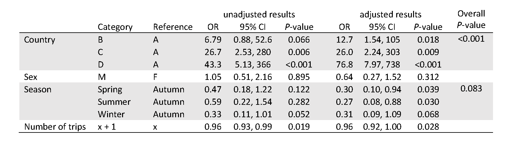
The data for this example are based on passenger arrival data collected by the Department of Agriculture as part of their routine screening of airline passengers arriving in Australia from 2013 to 2014. For each arrival, various passenger and travel characteristics are provided; a logistic regression analysis was performed on whether or not they were carrying material considered to pose a biosecurity risk (biosecurity risk material or BRM) and considered the impact of the passport country of the passenger, their sex, their historical number of trips, and the season of their arrival on Some results are presented in the table below:
More details about these data and the analysis described can be found here.
Interpreting odds ratios in logistic regression
Sometimes it can appear that the odds ratio and P-value results do not present a consistent picture across the explanatory variables. Why, for example, is the estimated odds ratio for the number of trips close to 1 when the P-value is similar to those for the various seasonal effects, which have much smaller odds ratios?
To interpret the odds ratios, we need to consider the measurement scale along with what might be considered a meaningful change on that scale, for each of the explanatory variables. In this way, we can consider the relative impact of the explanatory variables.
Recall the interpretation of the odds ratio for the number of trips: for each additional trip a passenger has taken, their odds of being found to be carrying BRM are estimated to decrease by a factor of 0.96 (or by 4%). However, the number of trips taken by an individual can vary from 1 to hundreds of trips. So perhaps the effect of one additional trip is not really a change that is of interest in this case. Our interpretation and understanding of these results may be helped if we undertake a rescaling of the number of trips variable.
Rescaling of explanatory variables
We will illustrate this idea for our example. Rather than considering the number of trips, we rescale this variable so that a one unit change is actually 10 additional trips. We can do this by dividing it by 10. It is best to make a new variable, to avoid confusion.
Here is the table of results including this new variable in place of the original number of trips.
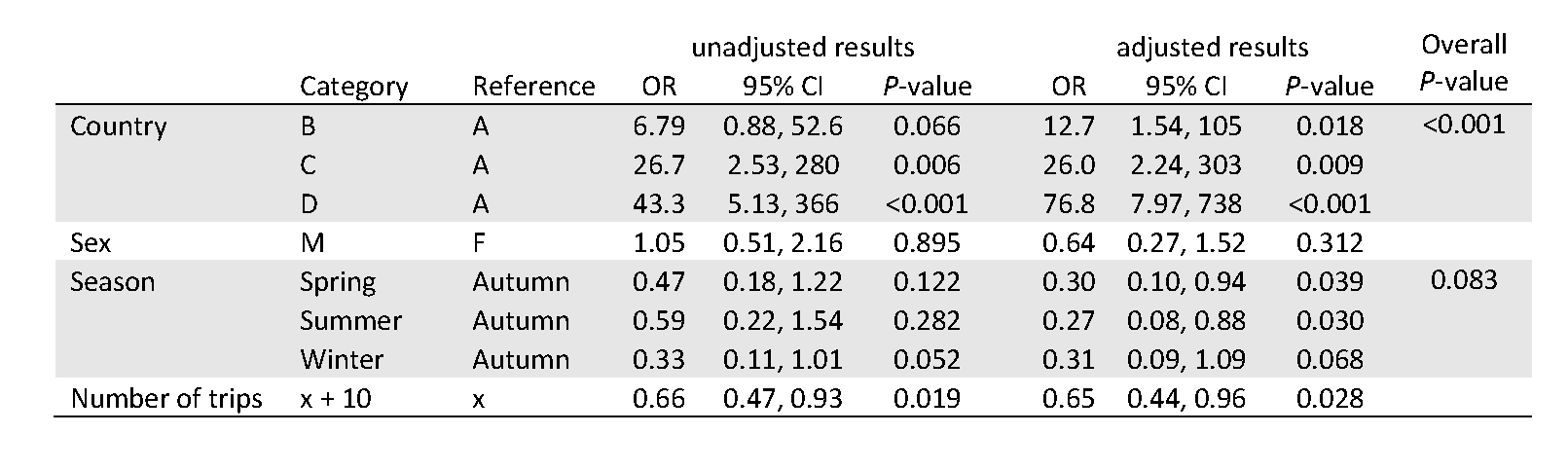
If you compare this with the original table above, you will see that the:
- P-values remain the same;
- odds ratio and confidence interval for the other variables are unchanged (as they should be, given we made no change to these variables);
- the odds ratios and confidence interval bounds for number of trips have changed’
- with the rescaling, for every 10 additional trips that a passenger has taken, their odds of being found to be carrying BRM are estimated to decrease by a factor 0.65 (or 35%).
This gives inferences for the impact of this variable for a more meaningful increment in the number of trips.
Direct rescaling of the coefficients
It is not necessary to calculate a rescaled explanatory variable and rerun your analysis to work out the odds ratio and confidence interval limits for a rescaled variable. The odds ratio and confidence interval limits can be rescaled directly. To do so, we need to scale the odds ratio in a multiplicative way, as logistic regression analysis is performed on a transformed scale. For example, the new odds ratio for a change of 10 trips is the original odds ratio to the power of 10. In the example, 0.9610=0.65.
As this can be tricky to think about and possible to get wrong, you can always calculate the rescaled variable and run the analysis again, as described above. Rescaling the variable also prevents errors introduced by rounding, particularly relevant for small odds ratios.
Changing the reference category
There are other ways we can sometimes improve the presentation of our model. For example, an odds ratio greater than 1 can often be easier to interpret than an odds ratio less than 1. The adjusted odds ratio of 12.7 in the first row of our first table indicates that we estimate that the odds of carrying BRM are 12.7 times higher for a passenger from Country B compared to Country A. However, for season, the odds of a passenger carrying BRW in winter are reported to be 0.31 times the odds for a passenger travelling in autumn. This is equivalent to saying that the odds are 3.23 times higher (1/0.31) in autumn compared to winter, which is a more natural way to consider the change in odds. We can simply invert the odds ratio to consider to reverse the category considered and the reference.
We can simply invert the values in the table directly. The confidence intervals can also be inverted in the same way, noting that the upper and lower limits then need to be reversed. However, it is usually preferable to formally change the reference category in software if you can. For example, in R, since season was coded as a factor, you can change the reference category using the following code:

The following table presents the seasons results with “winter” as the reference level.
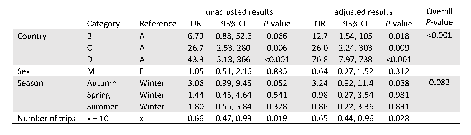
For the comparison between winter and autumn, the P-value remains the same but the inverted odds ratio is now 3.24. Note that this is slightly different to the inverted odds ratio from the table (1/0.31=3.23), due to rounding.
While software defaults to presenting all results with reference to a single factor level, it may be helpful to include every pairwise comparison in the same table.
Of course, there can be good reasons for choosing the reference category, such as treatments compared to a control, which may be a higher priority than presenting odds ratios greater than 1.