One way ANOVA
AN EXAMPLE
This example uses a dataset called ‘chickwts’. It is one of the inbuilt datasets provided in R software, and is popular for illustrating methods of one-way analysis of variance.
Chicks were fed one of six diets with different types of protein sources. The outcome of the study on chick growth was the weight in grams at six weeks of age. The categorical explanatory variable or factor is protein source. The interest is the effect of protein source (diet) on chick weight.
These are the six protein sources used in the diets. Horsebean, linseed oil mean, soybean oil meal and sunflower oil meal are all plant products. Meat meal and casein are animal products.
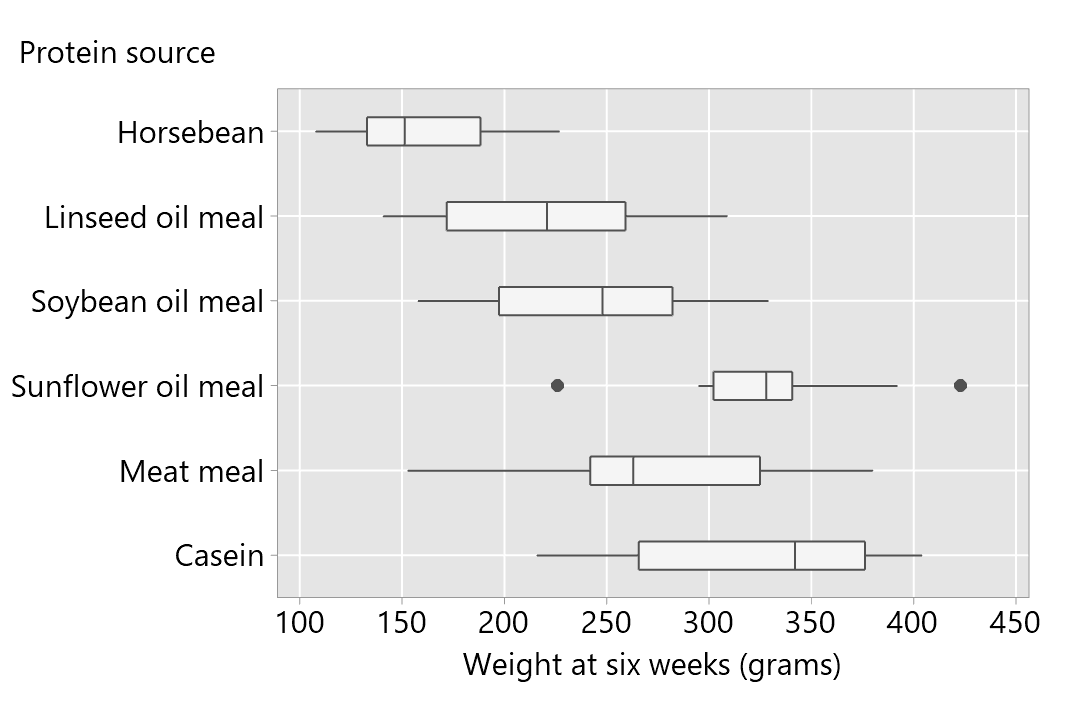
Here are boxplots of the data:
TAKING CARE WITH CONTEXT
This R dataset is an example where better care could have been taken in preserving the context of the data; see another example here. In the R documentation, the reference for the source of this dataset is:
- Anonymous (1948) Biometrika, 35, 214.
This is incorrect. The data were published in Biometrics in 1948, in volume 4(3) on page 214. The data were provided in a section of Biometrics called ‘Queries’, with a response from George W. Snedecor, a pioneer in applied statistics.
The correct reference is:
- Snedecor, G.W. (1948) 60. Query, Biometrics, 4(3), 213-215.
(It should be noted however that Snedecor did not collect the data.)
A QUERY?
The anonymous source, who provided the data, sent this query in to Biometrics. Snedecor provided an answer.
“I enclose data I have collected on chick growth and have indicated what appears to be four possible ways of showing the significance of the differences between the means obtained. My problem is one of how best to present these data and their implications in print. Your comments and suggestions … will be greatly appreciated. In a feeding trial with chicks designed to study the comparative feeding values of six protein supplements, fourteen chicks were used per lot to begin with. The birds were all of the same sex and age and were from the same flock. During the course of the experiment, some chicks died due to unknown cause.” (page 213)
It was indicated that all the diets had the same level of crude protein, and that the chicks receiving each diet were housed together.
Here we illustrate some approaches to reporting of the analysis of these data. The statistical analysis uses a one-way ANOVA, or equivalently, a linear model with one categorical explanatory variable. An appropriate report of the analysis may include summary statistics, the estimated effects with 95% confidence intervals, and P-values including a P-value is for a global test of the null hypothesis of no difference between true means for different levels of the explanatory factor.
The analysis of these data, with the methods illustrated here, assumes that: the chick weight observations are independent, the random errors arise from a Normal distribution, and the variance of the random errors is constant. A good analysis involves assessment of these assumptions, including examination of residual plots, and this may be discussed in a description of the statistical methods used or in the reporting of the results. As we will see, Snedecor had concerns about some of the assumptions.
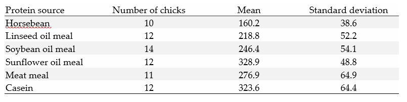
Here is an example of a summary table that provides descriptive statistics.
Table 1: Summary statistics for Chick weight at six weeks (g) by Protein source
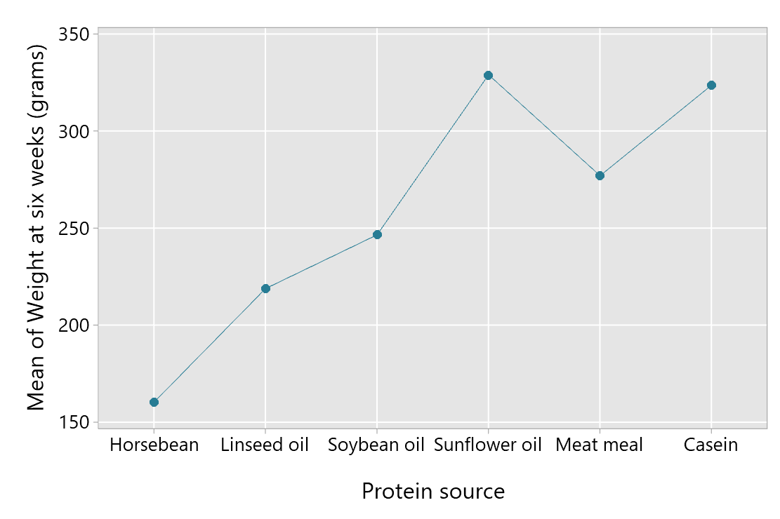
A plot of the means may also be useful:
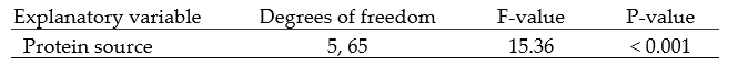
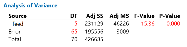
In some disciplines, the result of the hypothesis test is reported in a complete analysis of variance table. A more abbreviated report is suggested below. As here only one analysis is being reported, the hypothesis test result could easily (and preferably) be reported in the text. The table below is provided as an example that can be extended when multiple analyses are being reported.
Table 2: Statistical test from a one-way Anova model of Chick weight at six weeks (g)
The next aspect of reporting focuses on quantifying and interpreting the effect of the different sources of protein. There are different approaches to this, and the choice will depend, in part, on the design of the study. Two examples are provided to illustrate approaches to reporting.
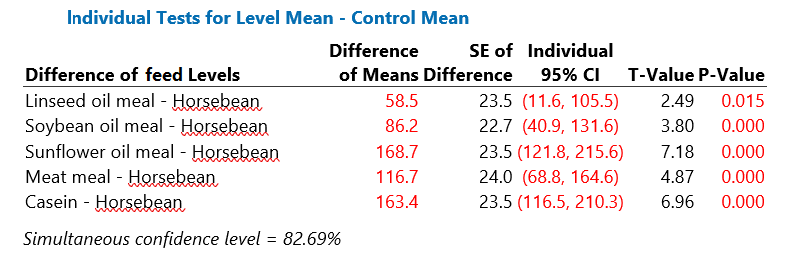
Snedecor suggests horsebean is a standard protein supplement. In this case, the effects of diet could be quantified by comparisons between horsebean and each of the other protein supplements. The inferences provided below are not adjusted for multiple comparisons.
Table 3: Mean Chick weights at 6 weeks (g): pairwise comparisons with the Horsebean supplement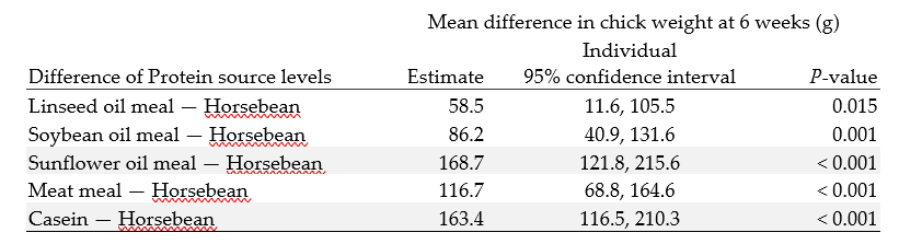
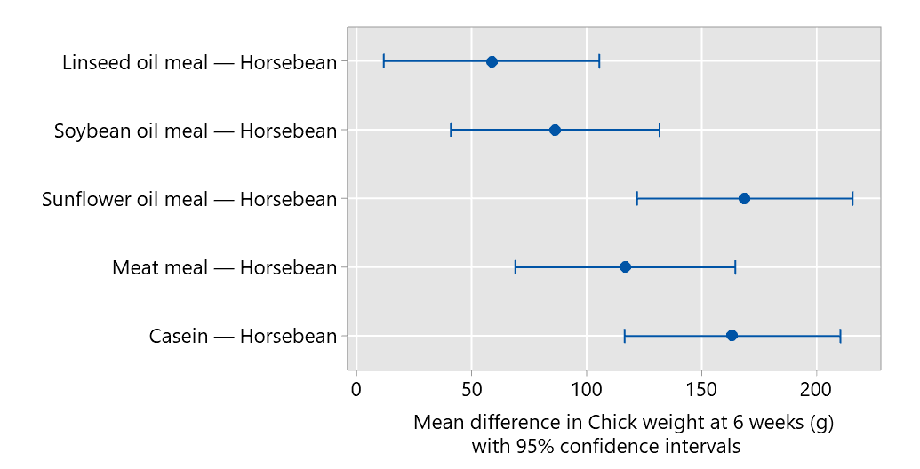
A plot of the comparisons is provided here:
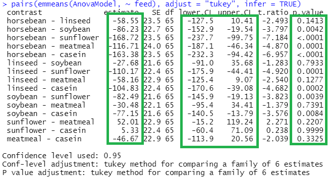
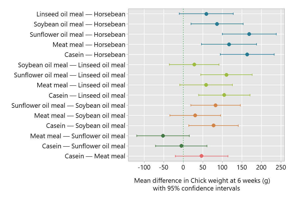
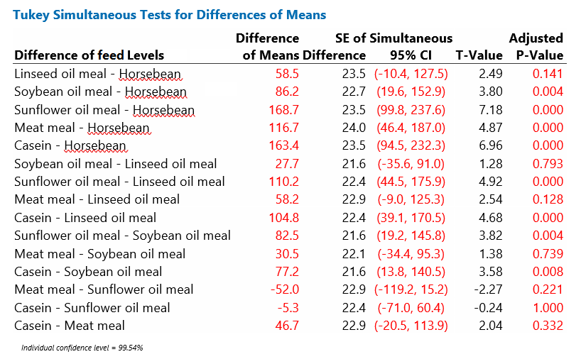
Another approach is to consider all the possible pairwise comparisons between the protein supplements; there will be 15 comparisons in all. When a factor has many levels, this can be complex to present. Careful layout of tables and graphs can help with this. The inferences illustrated below use Tukey’s method of adjustment for pairwise comparisons.
Table 4: Tukey’s Pairwise comparisons of mean Chick weights at 6 weeks (g) according to Protein source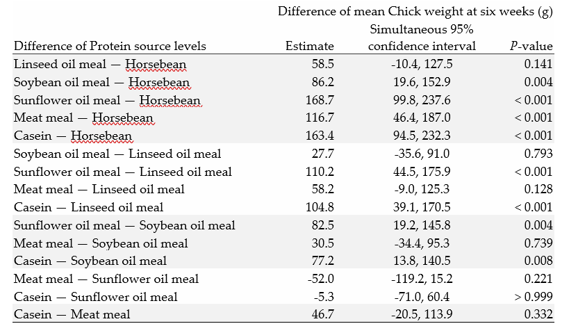
These comparisons are plotted below.
SNEDECOR’S RESPONSE
In his response, Snedecor suggested a set of comparisons. These were:
- Standard source (horsebean) versus other sources
- Vegetable sources versus animal
- Meat versus casein
- Two comparisons among vegetable sources
Reporting these comparisons would follow the principles described above.
However Snedecor was very critical of the way the study had been designed, and he suggested that there were “severe limitations”. These related to the chicks receiving a particular diet being housed together. They included:
- No effective replication of the diets, as chicks were treated as a group.
- Concern about whether the weights could be considered independent observations, an important assumption for using the statistical methods described here.
- The possibility that weight was related to intake, and that intake might be affected by the group housing.
- The confounding of environment and diet treatment which cannot be distinguished in this design.
In his final paragraph, Snedecor stated that “It is clearly my opinion that questions about tests of significance are of little weight as compared to those about the design and conduct of the experiment.” (page 214)
ANOTHER CONCERN
An additional concern, not mentioned in Snedecor’s answer, is the missing observations. There were 14 chicks in each diet group initially. Up to four chicks died before 6 weeks in each group apart from the soy bean meal where they all survived. The analysis will be compromised if the death of the chicks is related to the protein supplement they received.
SOFTWARE
In the examples of output for the statistical modelling from statistical software provided below, the variables are named as follows:
- Outcome: weight
- Explanatory variable: feed
The examples below assume some familiarity with the software you are using.
Minitab 19
The output from fitting a General Linear Model in Minitab is shown below, with the information used to construct Table 2 highlighted in red.
The pairwise comparisons, shown in Table 3:
The pairwise comparisons, shown in Table 4:
When you obtain the comparisons in Minitab, such as those above, you can request a plot as well.
R
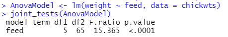
The code and output from R for obtaining the information summarised in Table 2 is shown below. The emmeans package is used, including the joint_tests() function to obtain the ANOVA below.
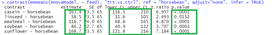
The code and output for the comparisons shown in Table 3:
The code and output for the comparisons, like those shown in Table 4, is below. Note that they are reversed from the results in Table 4: