Rescaling explanatory variables in linear regression
Introduction
Have you ever seen a very small estimated regression coefficient (e.g. 0.0023) for an explanatory variable that is reported with a very small P-value (e.g. P < 0.001)? Have you wondered how this is possible? This post discusses this phenomenon and some sensible approaches to dealing with it.
An example
This example uses data from the ‘SENIC’ project. SENIC refers to the Study on the Efficacy of Nosocomial Infection Control, carried out in the USA. The term ‘Nosocomial’ means hospital. Aims of the SENIC project included understanding the relationship between infection rate and hospital and patient characteristics.
A special issue of the American Journal of Epidemiology (Volume 111, Issue 5, May 1980) describes the SENIC project in detail.
The data used here were provided by a researcher to Kutner, M. H., Nachtsheim, C., Neter, J., & Li, W. (2005). Applied linear statistical models (5th ed.), Boston: McGraw-Hill. They are for a random sample of 111 hospitals from the larger sample of hospitals in the project. The variables are measured on hospitals and can, for example, refer to averages across patients in the hospital. The data here are for 1975-1976.
The outcome of interest is the hospital infection risk (on a percentage scale); this is the percentage of patients who experienced a hospital infection.
Three explanatory variables are considered:
- average age of patients (years)
- average length of stay (days)
- routine chest x-rays per 100; this is a ratio of the number of routine chest x-rays to the number of patients (excluding those with signs of pneumonia), multiplied by 100
Each of these variables could plausibly relate to the outcome; the last variable can be considered to be an indicator of hospital monitoring for potential infections.
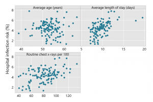
Here are scatterplots of the outcome and explanatory variables:
Interpreting the regression coefficients
A summary of the coefficients from a multiple linear regression model is:
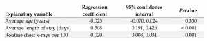
Sometimes people find results like this a little confusing — why, for example, are the regression coefficient and confidence interval limits so small for routine chest x-rays per 100 when the P-value is also small? Can that be the case?
Recall the interpretation of the regression coefficients: they indicate the predicted change in the outcome for a one-unit increase in the explanatory variable.
After adjustment for the other explanatory variables in the model, this means the model predicts:
- a decrease in hospital infection risk of 0.02% when average age increases by one year (the coefficient has a negative sign)
- an increase in hospital infection risk of 0.31% when average length of stay increases by one day
- an increase in hospital infection risk of 0.02% when routine chest x-rays per 100 increase by one.
Our interpretation and understanding of the regression coefficients will be helped if we consider the scale of the explanatory variables:
- average age ranged from 38.8 to 65.9 years
- average length of stay ranged from 6.7 to 19.6 days
- routine chest x-rays per 100 ranged from 39.6 to 133.5
You can see the ranges of these variables in the scatterplots, approximately.
A one-unit increase in the value of an explanatory variable corresponds to a change of:
- about 4% across the observed range for average age
- about 8% across the observed range for average length of stay
- about 1% across the observed range for routine chest x-rays per 100
So for routine chest x-rays per 100, the regression coefficient is indexing the predicted change in the outcome for a relatively small change (only about 1% of its range). It would be more useful to understand the effect of routine chest x-rays per 100 in terms of a more meaningful change across the scale.
This is where linear rescaling of the explanatory variable(s) can help.
Linear rescaling of explanatory variables
We illustrate this idea for average age and routine chest x-rays.
Rather than using average age in years, we could consider the average age in decades. We can calculate the new variable as the average age in years divided by ten.
Rather than using routine chest x-rays per 100, we could consider routine chest x-rays per 10. We can calculate the new variable as the routine chest x-rays per 100 divided by 10.
Here are the scatterplots of the outcome against the original and rescaled variables:
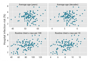
As the rescaling is linear the pattern of the association with the outcome does not change.
Now, we fit the multiple regression including the rescaled versions of average age and routine chest x-rays. The summary table is as follows:
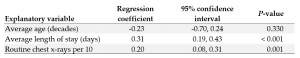
If you compare this with the original table, you will see that the:
- P-values remain the same
- regression coefficient and confidence interval for average length of stay are unchanged (as they should be, given we made no change to this variable)
- regression coefficient and confidence interval for average age (decades) are ten times those for average age (years)
- regression coefficient and confidence interval for routine chest x-rays per 10 are ten times those for routine chest x-rays per 100
This means the model predicts:
- a decrease in hospital infection risk of 0.23% when average age increases by ten years (the coefficient has a negative sign)
- an increase in hospital infection risk of 0.31% when average length of stay increases by one day
- an increase in hospital infection risk of 0.20% when routine chest x-rays per 10 increases by one.
Direct rescaling of the coefficients
The example above shows that it is not necessary to calculate a rescaled explanatory variable and rerun your analysis to work out the regression coefficient and confidence interval limits for a rescaled variable. The coefficient and confidence interval limits can be rescaled directly.
In our example, a regression coefficient of -0.023 for average age in years corresponds to -0.23 for age in decades. The explanatory variable is rescaled by dividing by ten; the regression coefficient and its associated confidence limits are rescaled by multiplying by ten.
When an explanatory variable would be rescaled using multiplication, the coefficients and confidence limits are rescaled by division by the same quantity.
But if you find this a little tricky to think about, you can always calculate the rescaled variable and run the analysis again.
A final note
The strategy discussed here is relevant to using a linear model, or regression, with continuous numerical explanatory variables, where these are included in the model as “main effects”. If interactions or cross-product terms are included in the model, things are less straightforward.