Managing native grasslands
Introduction
John and Ian were interested in finding a good way to maintain a diverse range of native flowering plants in Australian grasslands. The maintenance strategy needed to minimise weed invasion. He investigated different nutrient levels and mowing frequencies.
John and Ian worked on the study with Dr. Peter May from Burnley College; John worked at Burnley at the time, and Ian Shears works for the City of Melbourne. The project was funded by the Australian Flora Foundation.
The key question John and Ian wanted to answer was:
How do different nutrient levels and mowing frequencies affect the growth of native flower species in native grassland?
Timeline
- July 1997
- June 1998
-
Plots are planted
- February 1999
-
Data collection starts (First harvest)
- January 2000
-
Second harvest
- January 2001
-
Third harvest
- February 2001
-
Data analysis (Preliminary)
Background
Motivation for the study
Australia has some spectacular native flowering plants. Some of these are famous in particular locations, such as the wildflowers of Western Australia. Others are less prominent and were adversely affected by the introduction of sheep and cattle grazing in the early days of white settlement. These colourful plants grow among native grasses that compete with them, sometimes forming a canopy that threatens their survival.
In the wild, when the grasses are reduced by grazing and fire, the wildflowers within the grasslands are able to survive and flourish. It might be possible, particularly in controlled situations such as parks and gardens, to use management regimes for native grasslands that are conducive to the survival and growth of native wildflowers. Against this background, John and Ian set out to design a study that would evaluate different strategies for promoting the growth of wildflowers in Australian native grasslands.
Study report
In December 2006, John Delpratt and Ian Shears reported on the study to the Australia Flora Foundation.
Images from the trial
The photos below were taken at various times during the trial. They were taken by Ian Shears.
-
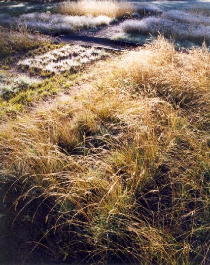
A recently mown plot in the foreground is beginning to re-grow. (It is the bottom left-hand plot in the Latin square.) The plot immediately behind was not mown; it is dominated by light coloured wallaby grass. This photo, figure 4 from the Delpratt and Shears report, was taken in March 1999. -
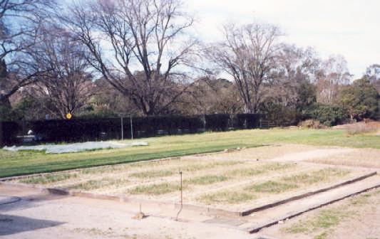
Newly constructed site with 16 plots, August 1998. Figure 1 from the Delpratt and Shears report. -
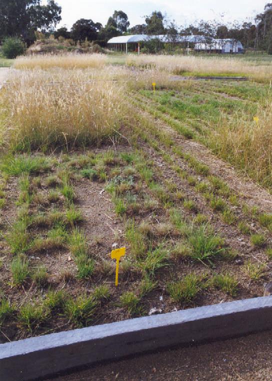
A close-up of a plot showing the central rectangle of kangaroo grass and wallaby grass, within which the native flowers are planted. The border of weeping grass is also evident. Figure 3 from the Delpratt and Shears report. -
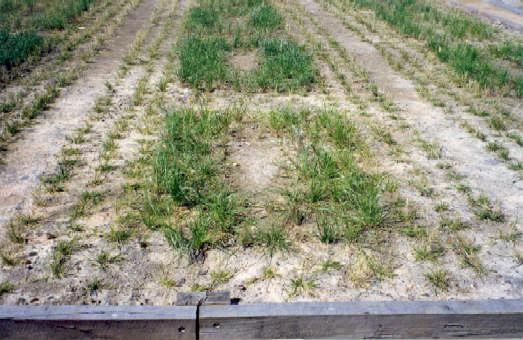
More-or-less continuous canopy cover formed by planted grasses in plots with added nitrogen. Figure 12 from the Delpratt and Shears report.
Study design
Latin square design
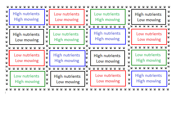
John and Ian’s study was carried out in an outdoor setting in the Field Station of the Burnley Campus of The University of Melbourne. Although a site that was as homogeneous as possible was chosen, characteristics (soil, weather, and so on) that are relevant to the growth of plants are likely to vary across any site. One way of dealing with this potential problem is to divide the site into blocks. John and Ian used a Latin square design; the site was divided into four rows and four columns, creating 16 plots. In a Latin square design, there are equal numbers of rows, columns, and treatments.
Treatments
Treatments are assigned at random within rows and columns. Each treatment occurs once in each row and once in each column. The treatment factor in the Latin square was made up of two factors: biennial (every 2 years) versus annual mowing, and high versus low levels of nutrients. Hence there was a 2 x 2 factorial structure among the treatments.
The video below was taken late in 2000, just before the third harvest. At this time, it was possible to distinguish the high and low nutrient plots by eye. High nutrient plots contain dense, light coloured wallaby grass which is highly visible. Low nutrient plots are darker and more sparse; they are dominated by dark coloured kangaroo grass and there is little wallaby grass.
Variables measured at mowing
Dry weight of each native flowering plant
Dry weight of each of three different grasses
Variables measured for each native flowering species
These measures were taken at irregular intervals.
- Number of plants with above-ground green tissue
- Number of plants in bud
- Number of plants in flower
- Number of plants in fruit
- Number of plants dropping seeds
Layout of individual plots
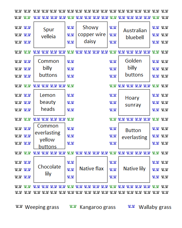
The layout below was used in each of the 16 plots in the Latin Square. The positions of the 12 native flowering plants in this layout were decided by random allocation. Kangaroo grass and wallaby grass were used to border the area in which each native was planted. Weeping grass was planted to separate the 16 plots in the Latin square. Each plot included the 12 different species of flowering natives and used three grasses as borders. Each plot was 1.7 metres long and 1.0 metre wide, excluding the border of weeping grass.
There is an unplanted area in the centre of each plot. This is deliberate; it allowed access to each plot for applying nutrients (where appropriate) and mowing. In each plot, 24 kangaroo grass plants, 72 wallaby grass plants and four of each of 12 native flowering species were planted.
Data collection
Protocol
| Soil preparation | Prepare 200 square metre area topped with weed-free, low-nutrient sub-soil of at least 30cm. |
|---|---|
| Plot establishment | Establish 16 plots in a 4 by 4 layout. Each plot is 2 square metres. Plant native grass, Microlaena stipoides, to establish a border each plot. |
| Plot layout | Randomly assign 12 native flowering plants to 12 planting trays. |
| Plot preparation | Plant each plot with a matrix of native grasses, Themeda triandra and Danthonia caespitosa, and 12 native flowering plants. |
| Nutrient treatment | Hand broadcast 10 grams per metre of ammonium nitrate on plots A and B. Repeat the treatment every two months. Plots C and D receive no nutrients. |
|---|---|
| Mowing regime | Plots are clipped to a height of 50mm by hand to simulate mowing. All plants are harvested, including the native grass bordering each plot. |
| Mowing treatment | For high-frequency mowing (plots A and C), harvest once a year. For low-frequency mowing (plots B and D), harvest once every two years. |
| Measuring dry weight | Separate each species of plant collected from each plot. Dry plants in oven at 80 degrees Celcius. Record dry weight in grams. |
Study log
| June, 1998 | All plots planted. |
|---|---|
| September, 1998 | Nutrients applied to plots A and B. |
| November, 1998 | Nutrients applied to plots A and B. |
| January, 1999 | Nutrients applied to plots A and B. |
| February, 1999 | Plots A and C harvested. |
| March, 1999 | Nutrients applied to plots A and B. |
| May, 1999 | Nutrients applied to plots A and B. |
| July, 1999 | Nutrients applied to plots A and B. |
| September, 1999 | Nutrients applied to plots A and B. |
| November, 1999 | Nutrients applied to plots A and B. |
|---|---|
| January, 2000 | All plots harvested; Nutrients applied to plots A and B. |
| March, 2000 | Nutrients applied to plots A and B. |
| May, 2000 | Nutrients applied to plots A and B. |
| July, 2000 | Nutrients applied to plots A and B. |
| September, 2000 | Nutrients applied to plots A and B. |
| November, 2000 | Nutrients applied to plots A and B. |
| January, 2001 | Plots A and C harvested; Nutrients applied to plots A and B. |
Analysis
Summary
John and Ian’s main interest was in the growth of the 12 different species of native flowers. There was great variety in the yields of the native flowers at the second harvest. Harvested yields for some species were very low because those species were dormant during the summer. However the mowing and nutrient treatments did influence yield for some species. The effects were different for different species of flowers. The treatments also had varying effects on the yield of the grasses.

Boxplots of yield in grams at the second harvest (n=16 for each boxplot).
Questions to consider
- Examine the boxplots shown above. Broadly, what kinds of analysis would you recommend for the various species?
- Choose a species for which there was variability in the dry weight. Provide a visual display to illustrate the variation in dry weights by treatment.
- Consider the assumptions required for analysing the Latin square design using a standard analysis of variance. For which species are these assumptions met? Produce a visual display to support your conclusions.
- Conduct a statistical analysis of the Latin square design (treatments, rows and columns) for one or more of the grass species. Write a brief summary of the results and include a visual display to illustrate the main findings.
- Investigate the effects of the mowing treatment and the nutrient treatment for native flower species that interests you. Write a brief summary of results and an explanation.
- Investigate the assumptions required for analysing the Latin square for three different species. What kind of strategies are appropriate in cases where the assumptions are not met? What kind of inferences can be made?
- For some species there is little variation in dry weight and only a small number of positive values observed. What kind of descriptive and inferential analyses would you consider for these species?
Data
Note that the data file only includes dry weight data from the second harvest. Although John’s primary interest was in the native flowers (species 3 to 14), he also recorded the dry weight of the three grasses (species 1, 2 and 15).
Definition of species and treatment variables in data file
| Species Number | Species name | Common name |
|---|---|---|
| 1 | Austrodanthonia caespitosa | Wallaby grass |
| 2 | Themeda triandra | Kangaroo grass |
| 3 | Wahlenbergia stricta | Australian bluebell |
| 4 | Pycnosorus chrysanthes | Golden billy buttons |
| 5 | Leucochrysum albicans | Hoary sunray |
| 6 | Helichrysum scorpiodes | Button everlasting |
| 7 | Bulbine bulbosa | Native lily |
| 8 | Linum marginale | Native flax |
| 9 | Arthropodium strictum | Chocolate lily |
| 10 | Chrysocephalum apiculatum | Common everlasting yellow buttons |
| 11 | Calocephalus citreus | Lemon beauty heads |
| 12 | Craspedia variabilis | Common billy-buttons |
| 13 | Velleia paradoxa | Spur velleia |
| 14 | Podolepis jaceoides | Showy copper-wire daisy |
| 15 | Microlaena stipoides | Weeping grass |
| Combined Nutrient and Mowing treatment | |
|---|---|
| 1 | Treatment A – high nutrients and annual mowing |
| 2 | Treatment B – high nutrients and biennial mowing |
| 3 | Treatment C – low nutrients and annual mowing |
| 4 | Treatment D – low nutrients and biennial mowing |
Definition of remaining variables in data file
| Row | Row in latin square |
|---|---|
| Column | Column in latin square |
| Weight | Dry weight in grams |
| Mowing | Mowing treatment: 1 = annual, 0 = biennial |
| Nutrient | Nutrient treatment: 1 = high nutrients, 0 = low nutrients |
| T1 | Treatment (Species 1) |
| R1 | Row in latin square (Species 1) |
| C1 | Column in latin square (Species 1) |
| W1 | Dry weight in grams of Species 1 |
| M1 | Mowing treatment (Species 1) |
| N1 | Nutrient treatment (Species 1) |
| T2 | Treatment (Species 2) |
| R2 | Row in latin square (Species 2) |
| C2 | Column in latin square (Species 2) |
| W2 | Dry weight in grams of Species 2 |
| M2 | Mowing treatment (Species 2) |
|---|---|
| N2 | Nutrient treatment (Species 2) |
| T8 | Treatment (Species 8) |
| R8 | Row in latin square (Species 8) |
| C8 | Column in latin square (Species 8) |
| W8 | Dry weight in grams of Species 8 |
| M8 | Mowing treatment (Species 8) |
| N8 | Nutrient treatment (Species 8) |
| T15 | Treatment (Species 15) |
| R15 | Row in latin square (Species 15) |
| C15 | Column in latin square (Species 15) |
| W15 | Dry weight in grams of Species 15 |
| M15 | Mowing treatment (Species 15) |
| N15 | Nutrient treatment (Species 15) |