Design and data collection
Study design
Latin square design
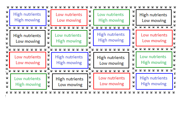
John and Ian’s study was carried out in an outdoor setting in the Field Station of the Burnley Campus of The University of Melbourne. Although a site that was as homogeneous as possible was chosen, characteristics (soil, weather, and so on) that are relevant to the growth of plants are likely to vary across any site. One way of dealing with this potential problem is to divide the site into blocks. John and Ian used a Latin square design; the site was divided into four rows and four columns, creating 16 plots. In a Latin square design, there are equal numbers of rows, columns, and treatments.
Treatments
Treatments are assigned at random within rows and columns. Each treatment occurs once in each row and once in each column. The treatment factor in the Latin square was made up of two factors: biennial (every 2 years) versus annual mowing, and high versus low levels of nutrients. Hence there was a 2 x 2 factorial structure among the treatments.
The video below was taken late in 2000, just before the third harvest. At this time, it was possible to distinguish the high and low nutrient plots by eye. High nutrient plots contain dense, light coloured wallaby grass which is highly visible. Low nutrient plots are darker and more sparse; they are dominated by dark coloured kangaroo grass and there is little wallaby grass.
Variables measured at mowing
Dry weight of each native flowering plant
Dry weight of each of three different grasses
Variables measured for each native flowering species
These measures were taken at irregular intervals.
- Number of plants with above-ground green tissue
- Number of plants in bud
- Number of plants in flower
- Number of plants in fruit
- Number of plants dropping seeds
Layout of individual plots
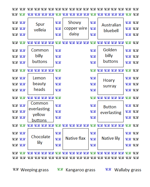
The layout below was used in each of the 16 plots in the Latin Square. The positions of the 12 native flowering plants in this layout were decided by random allocation. Kangaroo grass and wallaby grass were used to border the area in which each native was planted. Weeping grass was planted to separate the 16 plots in the Latin square. Each plot included the 12 different species of flowering natives and used three grasses as borders. Each plot was 1.7 metres long and 1.0 metre wide, excluding the border of weeping grass.
There is an unplanted area in the centre of each plot. This is deliberate; it allowed access to each plot for applying nutrients (where appropriate) and mowing. In each plot, 24 kangaroo grass plants, 72 wallaby grass plants and four of each of 12 native flowering species were planted.
Data collection
Protocol
| Soil preparation | Prepare 200 square metre area topped with weed-free, low-nutrient sub-soil of at least 30cm. |
|---|---|
| Plot establishment | Establish 16 plots in a 4 by 4 layout. Each plot is 2 square metres. Plant native grass, Microlaena stipoides, to establish a border each plot. |
| Plot layout | Randomly assign 12 native flowering plants to 12 planting trays. |
| Plot preparation | Plant each plot with a matrix of native grasses, Themeda triandra and Danthonia caespitosa, and 12 native flowering plants. |
| Nutrient treatment | Hand broadcast 10 grams per metre of ammonium nitrate on plots A and B. Repeat the treatment every two months. Plots C and D receive no nutrients. |
|---|---|
| Mowing regime | Plots are clipped to a height of 50mm by hand to simulate mowing. All plants are harvested, including the native grass bordering each plot. |
| Mowing treatment | For high-frequency mowing (plots A and C), harvest once a year. For low-frequency mowing (plots B and D), harvest once every two years. |
| Measuring dry weight | Separate each species of plant collected from each plot. Dry plants in oven at 80 degrees Celcius. Record dry weight in grams. |
Study log
| June, 1998 | All plots planted. |
|---|---|
| September, 1998 | Nutrients applied to plots A and B. |
| November, 1998 | Nutrients applied to plots A and B. |
| January, 1999 | Nutrients applied to plots A and B. |
| February, 1999 | Plots A and C harvested. |
| March, 1999 | Nutrients applied to plots A and B. |
| May, 1999 | Nutrients applied to plots A and B. |
| July, 1999 | Nutrients applied to plots A and B. |
| September, 1999 | Nutrients applied to plots A and B. |
| November, 1999 | Nutrients applied to plots A and B. |
|---|---|
| January, 2000 | All plots harvested; Nutrients applied to plots A and B. |
| March, 2000 | Nutrients applied to plots A and B. |
| May, 2000 | Nutrients applied to plots A and B. |
| July, 2000 | Nutrients applied to plots A and B. |
| September, 2000 | Nutrients applied to plots A and B. |
| November, 2000 | Nutrients applied to plots A and B. |
| January, 2001 | Plots A and C harvested; Nutrients applied to plots A and B. |